[14]:
from mind_the_gaps.lightcurves import GappyLightcurve
from mind_the_gaps.gpmodelling import GPModelling
from mind_the_gaps.models import BendingPowerlaw, Lorentzian, SHO, Matern32, Jitter
from mind_the_gaps.simulator import Simulator
import numpy as np
import matplotlib.pyplot as plt
import celerite, corner
from scipy.stats import percentileofscore

cpus = 15 # set the number of cores for parallelization
np.random.seed(10)
Tutorial: PPPP
Case of No period
Define parameters for lightcurve simulation
[15]:
times  = np.arange(0, 1000)
dt = np.diff(times)[0]

mean = 100

#A = (mean * 0.1) ** 2 # variance of the lorentzian
#Q = 80
variance_drw = (mean * 0.1) ** 2  # variance of the DRW (bending powerlaw)
w_bend = 2 * np.pi / 20 # angular frequency of the DRW or Bending Powerlaw

# define the PSD model
psd_model = BendingPowerlaw(variance_drw, w_bend)
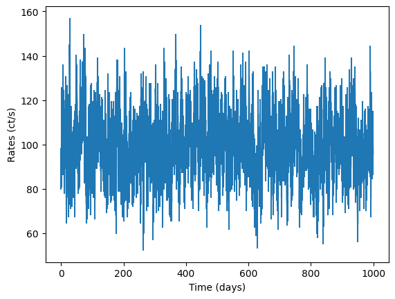
Simulate lightcurve
[16]:
# create simulator object
simulator = Simulator(psd_model, times, np.ones(len(times)) * dt, mean, pdf="Gaussian",
                     extension_factor=2)
# simulate noiseless count rates from the PSD, make the initial lightcurve 2 times as long as the original times
countrates = simulator.generate_lightcurve()
# add (Poisson) noise
noisy_countrates, dy = simulator.add_noise(countrates)

input_lc = GappyLightcurve(times, noisy_countrates, dy, exposures=dt)

fig = plt.figure()
plt.errorbar(times, noisy_countrates, yerr=dy)
plt.xlabel("Time (days)")
plt.ylabel("Rates (ct/s)")
[16]:
Text(0, 0.5, 'Rates (ct/s)')
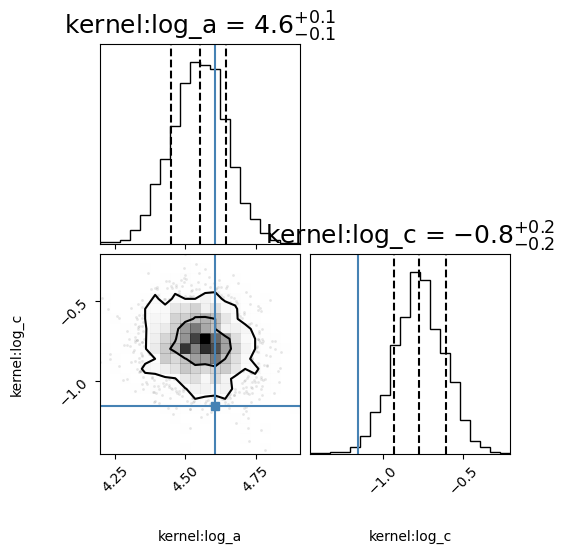
Define null hypothesis
[17]:
# null
bounds_drw = dict(log_a=(-10, 50), log_c=(-10, 10))
# you can use RealTerm from celerite or DampedRandomWalk from models.celerite_models
null_kernel = celerite.terms.RealTerm(log_a=np.log(variance_drw), log_c=np.log(w_bend), bounds=bounds_drw)
null_model = GPModelling(input_lc, null_kernel)
print("Deriving posteriors for null model")
null_model.derive_posteriors(max_steps=50000, fit=True, cores=cpus)
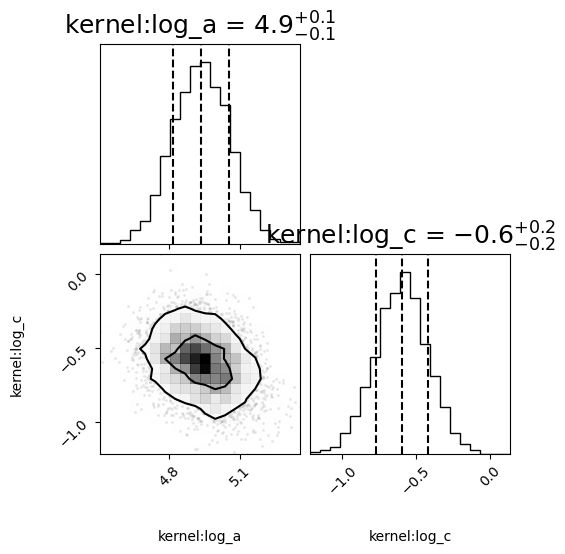
corner_fig = corner.corner(null_model.mcmc_samples, labels=null_model.gp.get_parameter_names(), title_fmt='.1f',
quantiles=[0.16, 0.5, 0.84], show_titles=True, truths=[np.log(variance_drw), np.log(w_bend)],
title_kwargs={"fontsize": 18}, max_n_ticks=3, labelpad=0.08,
levels=(1 - np.exp(-0.5), 1 - np.exp(-0.5 * 2 ** 2))) # plots 1 and 2 sigma levels
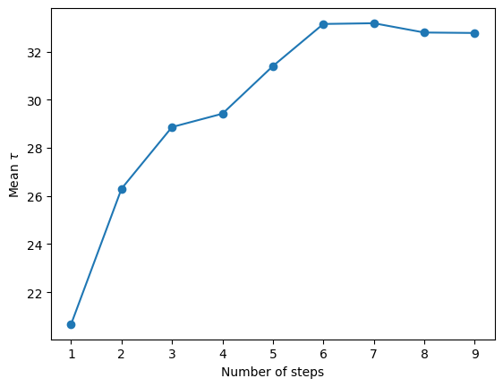
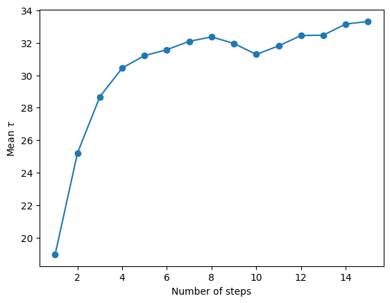
autocorr = null_model.autocorr
fig = plt.figure()
n = np.arange(1, len(autocorr) + 1)
plt.plot(n, autocorr, "-o")
plt.ylabel("Mean $\\tau$")
plt.xlabel("Number of steps")
plt.savefig("autocorr.png", dpi=100)
Deriving posteriors for null model
9%|███▎ | 4500/50000 [00:20<03:25, 221.26it/s]
Convergence reached after 4500 samples!
Define alternative model
[18]:
P = 10 # period of the QPO
w = 2 * np.pi / P
# Define starting parameters
log_variance_qpo = np.log(variance_drw)
Q = 80 # coherence
log_c = np.log(0.5 * w/Q)
log_d = np.log(w)
print(f"log variance of the QPO: {log_variance_qpo:.2f}, log_c: {log_c:.2f}, log omega: {log_d:.2f}")
bounds_qpo = dict(log_a=(-10, 50), log_c=(-10, 10), log_d=(-5, 5))
# You can also use Lorentzian from models.celerite_models (which is defined in terms of variance, Q and omega)
alternative_kernel = celerite.terms.ComplexTerm(log_a=log_variance_qpo, log_c=log_c, log_d=log_d, bounds=bounds_qpo) \
+ celerite.terms.RealTerm(log_a=np.log(variance_drw), log_c=np.log(w_bend), bounds=bounds_drw)
alternative_model = GPModelling(input_lc, alternative_kernel)
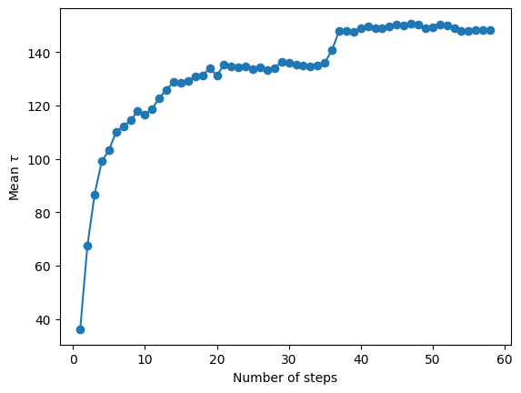
print("Deriving posteriors for alternative model")
alternative_model.derive_posteriors(max_steps=50000, fit=True, cores=cpus)
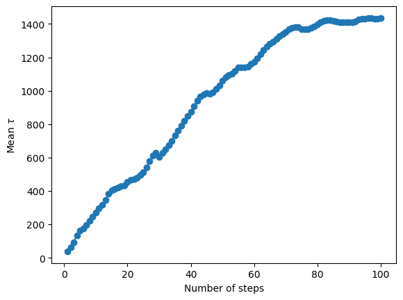
autocorr = alternative_model.autocorr
fig = plt.figure()
n = np.arange(1, len(autocorr) + 1)
plt.plot(n, autocorr, "-o")
plt.ylabel("Mean $\\tau$")
plt.xlabel("Number of steps")
plt.savefig("autocorr.png", dpi=100)
corner_fig = corner.corner(alternative_model.mcmc_samples, labels=alternative_model.gp.get_parameter_names(),
title_fmt='.1f',
quantiles=[0.16, 0.5, 0.84], show_titles=True,
title_kwargs={"fontsize": 18}, max_n_ticks=3, labelpad=0.08,
levels=(1 - np.exp(-0.5), 1 - np.exp(-0.5 * 2 ** 2))) # plots 1 and 2 sigma levels
log variance of the QPO: 4.61, log_c: -5.54, log omega: -0.46
Deriving posteriors for alternative model
58%|████████████████████▉ | 29000/50000 [02:57<02:08, 163.08it/s]
Convergence reached after 29000 samples!
Generate lightcurves from null hypothesis posteriors
[19]:
Nsims = 100 # typically 10,000
lcs = null_model.generate_from_posteriors(Nsims, cpus=cpus)
print("Done!")
Done!
Fit the lightcurves with both null and alternative models
[20]:
likelihoods_null = []
likelihoods_alt = []

for i, lc in enumerate(lcs):
    print("Processing lightcurve %d/%d" % (i + 1, len(lcs)), end="\r")

    # Run a small MCMC to make sure we find the global maximum of the likelihood
    # ideally we'd probably want to run more samples
    null_modelling = GPModelling(lc, null_kernel)
    null_modelling.derive_posteriors(fit=True, cores=cpus, walkers=2 * cpus, max_steps=500, progress=False)
    likelihoods_null.append(null_modelling.max_loglikelihood)
    alternative_modelling = GPModelling(lc, alternative_kernel)
    alternative_modelling.derive_posteriors(fit=True, cores=cpus, walkers=2 * cpus, max_steps=500,
                                            progress=False)
    likelihoods_alt.append(alternative_modelling.max_loglikelihood)


print("\nDone!")
Processing lightcurve 100/100
Done!
Calculate T_LRT distribution and compare with the observed value
[21]:
plt.figure()
T_dist = -2 * (np.array(likelihoods_null) - np.array(likelihoods_alt))
print(T_dist)
plt.hist(T_dist, bins=10)
T_obs = -2 * (null_model.max_loglikelihood - alternative_model.max_loglikelihood)
print("Observed LRT_stat: %.3f" % T_obs)
perc = percentileofscore(T_dist, T_obs)
print("p-value: %.4f" % (1 - perc / 100))
plt.axvline(T_obs, label="%.2f%%" % perc, ls="--", color="black")

sigmas = [95, 99.7]
colors= ["red", "green"]
for i, sigma in enumerate(sigmas):
    plt.axvline(np.percentile(T_dist, sigma), ls="--", color=colors[i])
plt.legend()
#plt.axvline(np.percentile(T_dist, 99.97), color="green")
plt.xlabel("$T_\\mathrm{LRT}$")

#plt.savefig("LRT_statistic.png", dpi=100)
[ 7.30563401  2.94625081 14.75289871 10.52743179  7.74959716  5.8785983
  3.20299343  2.38046508  3.17474049  3.81860381  3.88019518  7.29723268
  4.85259113  2.98080648  3.39319164  3.59714561  9.8966823   3.88529402
  3.99449269  2.46099526  5.25084205  6.16162681  1.81614045  5.28701198
  4.12006926  2.91897357  4.83303362  4.23900587  5.63685765  4.79250275
  6.79145503  3.9150156   3.43018229  2.02956163  7.65994804  2.46595943
  3.12158707  4.40684836  2.83288652  4.50240423  3.76856325  3.85560336
  1.15337875  5.83975122  2.18666619  5.18070065  8.05677747  4.84126984
  1.24310117  6.4208726   4.52304552  6.07630189  2.39039578  2.89344625
  4.05528121  0.97658978  3.67092644  5.27092732 14.10653823  3.30498505
  4.80172475  5.6401755   2.90531107  3.16989271  2.42755883  4.12166258
  7.06811315  1.86199878 14.64522556  2.1870361   7.30821463  6.96152377
 13.27480981  4.73065428  3.46582211  2.32111937  6.57667026 11.72752958
  7.44425621  2.78618805  2.39949132  9.3003771   6.34826339  3.64166206
  4.0817636   6.20204133  3.99324566  1.73804533  1.79097601  3.56539597
  5.19618946  4.82505414  5.38537736  4.90753979  4.43595841  1.76022901
  5.13745067  6.53876006  3.56190523  2.97618685]
Observed LRT_stat: 5.257
p-value: 0.3200
[21]:
Text(0.5, 0, '$T_\\mathrm{LRT}$')
We see the p-value to reject the null hypothesis is fairly low, indicating there is no signal in this data, as expected
Case with Period
Simulate lightcurve
[7]:
times  = np.arange(0, 500)
dt = np.diff(times)[0]

mean = 100

P = 10 # period of the QPO
w_qpo = 2 * np.pi / P
w_bend = 2 * np.pi / 20 # angular frequency of the DRW or Bending Powerlaw
# Define starting parameters
variance_drw = (mean * 0.1) ** 2  # variance of the DRW (bending powerlaw)
variance_qpo = variance_drw # let's assume same variance for the QPO and the DRW

Q = 80 # coherence

psd_model = Lorentzian(variance_qpo, Q, w_qpo) + BendingPowerlaw(variance_drw, w_bend)
[8]:
simulator = Simulator(psd_model, times, np.ones(len(times)) * dt, mean, pdf="Gaussian", max_iter=500)
rates = simulator.generate_lightcurve()
noisy_rates, dy = simulator.add_noise(rates)
input_lc = GappyLightcurve(times, noisy_rates, dy, exposures=dt)
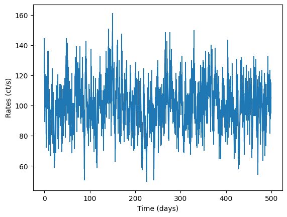
fig = plt.figure()
plt.errorbar(times, noisy_rates, yerr=dy)
plt.xlabel("Time (days)")
plt.ylabel("Rates (ct/s)")
[8]:
Text(0, 0.5, 'Rates (ct/s)')
Define null hypothesis
[9]:
bounds_drw = dict(log_a=(-10, 50), log_c=(-10, 10))
# null
null_kernel = celerite.terms.RealTerm(log_a=np.log(variance_drw), log_c=np.log(w_bend), bounds=bounds_drw)
null_model = GPModelling(input_lc, null_kernel)
print("Deriving posteriors for null model")
null_model.derive_posteriors(max_steps=50000, fit=True, cores=cpus)

corner_fig = corner.corner(null_model.mcmc_samples, labels=null_model.gp.get_parameter_names(), title_fmt='.1f',
                            quantiles=[0.16, 0.5, 0.84], show_titles=True,
                            title_kwargs={"fontsize": 18}, max_n_ticks=3, labelpad=0.08,
                            levels=(1 - np.exp(-0.5), 1 - np.exp(-0.5 * 2 ** 2))) # plots 1 and 2 sigma levels

autocorr = null_model.autocorr
fig = plt.figure()
n = np.arange(1, len(autocorr) + 1)
plt.plot(n, autocorr, "-o")
plt.ylabel("Mean $\\tau$")
plt.xlabel("Number of steps")
plt.savefig("autocorr.png", dpi=100)
Deriving posteriors for null model
15%|█████▌ | 7500/50000 [00:30<02:50, 248.54it/s]
Convergence reached after 7500 samples!
Define alternative model
[10]:
log_c = np.log(0.5 * w_qpo/Q)
log_d = np.log(w_qpo)
bounds_qpo = dict(log_a=(-10, 50), log_c=(-10, 10), log_d=(-5, 5))
# again you may use the Lorentzian from models.celerite_models
alternative_kernel = celerite.terms.ComplexTerm(log_a=np.log(variance_qpo), log_c=log_c,
log_d=np.log(w_bend), bounds=bounds_qpo) \
+ celerite.terms.RealTerm(log_a=np.log(variance_drw), log_c=np.log(w_bend), bounds=bounds_drw)
alternative_model = GPModelling(input_lc, alternative_kernel)
print("Deriving posteriors for alternative model")
alternative_model.derive_posteriors(max_steps=50000, fit=True, cores=cpus)
autocorr = alternative_model.autocorr
fig = plt.figure()
n = np.arange(1, len(autocorr) + 1)
plt.plot(n, autocorr, "-o")
plt.ylabel("Mean $\\tau$")
plt.xlabel("Number of steps")
plt.savefig("autocorr.png", dpi=100)
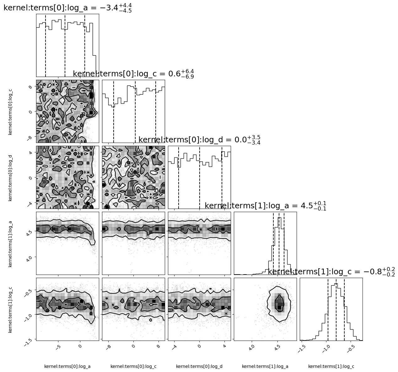
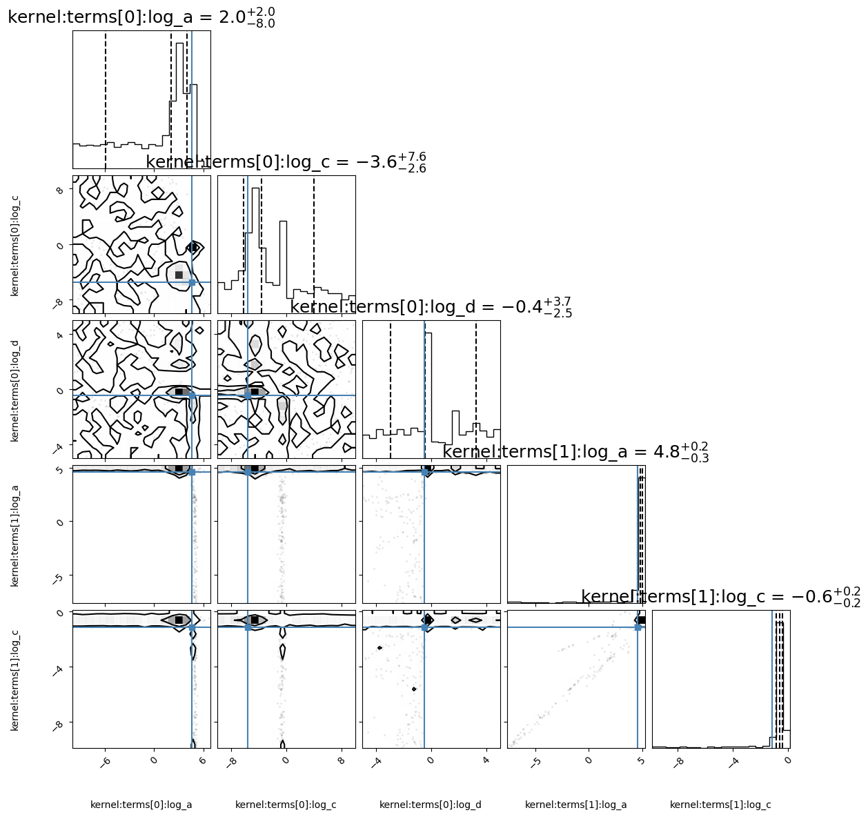
corner_fig = corner.corner(alternative_model.mcmc_samples, labels=alternative_model.gp.get_parameter_names(), title_fmt='.1f',
quantiles=[0.16, 0.5, 0.84], show_titles=True,
truths=[np.log(variance_qpo), log_c, log_d, np.log(variance_drw), np.log(w_bend)],
title_kwargs={"fontsize": 18}, max_n_ticks=3, labelpad=0.08,
levels=(1 - np.exp(-0.5), 1 - np.exp(-0.5 * 2 ** 2))) # plots 1 and 2 sigma levels
Deriving posteriors for alternative model
100%|████████████████████████████████████| 50000/50000 [04:52<00:00, 170.70it/s]
Generate lightcurves with null hypothesis posteriors
[11]:
Nsims = 100 # typically 10,000
lcs = null_model.generate_from_posteriors(Nsims, cpus=cpus)
print("Done!")
Done!
Fit the lightcurves with both null and alternative models
[12]:
likelihoods_null = []
likelihoods_alt = []

for i, lc in enumerate(lcs):
    print("Processing lightcurve %d/%d" % (i + 1, len(lcs)), end="\r")
    #fig = plt.figure()
    #plt.errorbar(lc.times, lc.y, lc.dy)
    #plt.xlabel("Time (days)")
    #plt.ylabel("Rate (ct/s)")
    #plt.savefig("%d.png" % i, dpi=100)

    # Run a small MCMC to make sure we find the global maximum of the likelihood
    # ideally we'd probably want to run more samples
    null_modelling = GPModelling(lc, null_kernel)
    null_modelling.derive_posteriors(fit=True, cores=cpus, walkers=2 * cpus, max_steps=500, progress=False)
    likelihoods_null.append(null_modelling.max_loglikelihood)
    alternative_modelling = GPModelling(lc, alternative_kernel)
    alternative_modelling.derive_posteriors(fit=True, cores=cpus, walkers=2 * cpus, max_steps=500,
                                            progress=False)
    likelihoods_alt.append(alternative_modelling.max_loglikelihood)


print("\nDone!")
Processing lightcurve 100/100
Done!
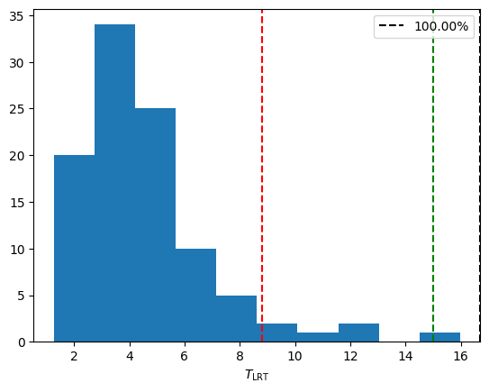
Calculate T_LRT distribution and compare with the observed value
[13]:
plt.figure()
T_dist = -2 * (np.array(likelihoods_null) - np.array(likelihoods_alt))
print(T_dist)
plt.hist(T_dist, bins=10)
T_obs = -2 * (null_model.max_loglikelihood - alternative_model.max_loglikelihood)
print("Observed LRT_stat: %.3f" % T_obs)
perc = percentileofscore(T_dist, T_obs)
print("p-value: %.4f" % (1 - perc / 100))
plt.axvline(T_obs, label="%.2f%%" % perc, ls="--", color="black")

sigmas = [95, 99.7]
colors= ["red", "green"]
for i, sigma in enumerate(sigmas):
    plt.axvline(np.percentile(T_dist, sigma), ls="--", color=colors[i])
plt.legend()
#plt.axvline(np.percentile(T_dist, 99.97), color="green")
plt.xlabel("$T_\\mathrm{LRT}$")

#plt.savefig("LRT_statistic.png", dpi=100)
[ 3.34906363 4.18603532 3.94396794 6.59518162 3.75650583 6.41527212
4.12079241 2.2515247 4.61438882 3.39965337 5.85466669 4.97434851
2.04255673 7.2018184 3.3057323 3.05963089 5.36061088 4.63561244
4.68763001 1.8914104 3.35164567 7.31447309 4.95433573 4.870965
2.93939517 5.55624968 7.22747865 4.19442597 2.40208188 4.19819722
2.08699125 5.99205782 3.26515473 3.65610264 3.466431 2.9348864
3.65870043 4.46798045 6.37269356 4.51377118 5.00974449 5.2878181
2.31384422 3.63255857 4.3254309 2.25674137 4.48274934 2.01117949
5.42155543 2.87991697 3.86360599 1.34082161 2.50945507 8.7816284
5.18318131 4.99904061 1.28062966 3.80425961 3.30724398 12.66112865
1.35389463 4.23576378 4.65620595 9.27455938 4.3138121 2.62993643
3.79278311 5.13349003 3.19733257 2.85958733 1.71209452 8.13522894
2.87108174 2.35853654 5.23669427 2.747617 15.97494691 11.79352313
2.917152 6.47973122 4.52182191 6.8260283 10.1096783 2.30888727
2.91636732 3.98779261 1.89947046 6.45497382 4.59613903 5.5530016
3.74590913 2.5545625 3.08670366 1.27278326 2.28363779 3.62572606
7.71704321 5.948798 3.78721488 6.08987315]
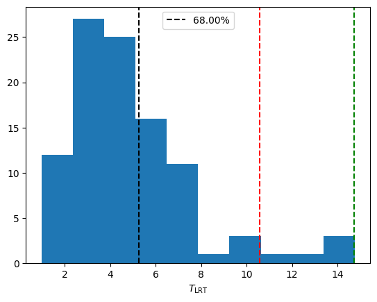
Observed LRT_stat: 16.689
p-value: 0.0000
[13]:
Text(0.5, 0, '$T_\\mathrm{LRT}$')
[ ]: